1
2
3
4
5
6
7
8
9
10
11
12
13
14
15
16
17
18
19
20
21
22
23
24
25
26
27
28
29
30
31
32
33
| clear;
close all;
clc;
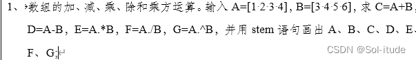
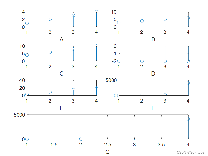
A=[1 2 3 4];
B=[3 4 5 6];
C=A+B;
D=A-B;
E=A.*B
F=A./B
F=A.^B
G=A.^B
subplot(4,2,1)
stem(A)
xlabel('A')
subplot(4,2,2)
stem(B)
xlabel('B')
subplot(4,2,3)
stem(C)
xlabel('C')
subplot(4,2,4)
stem(D)
xlabel('D')
subplot(4,2,5)
stem(E)
xlabel('E')
subplot(4,2,6)
stem(F)
xlabel('F')
subplot(4,2,[7,8])
stem(G)
xlabel('G')
|
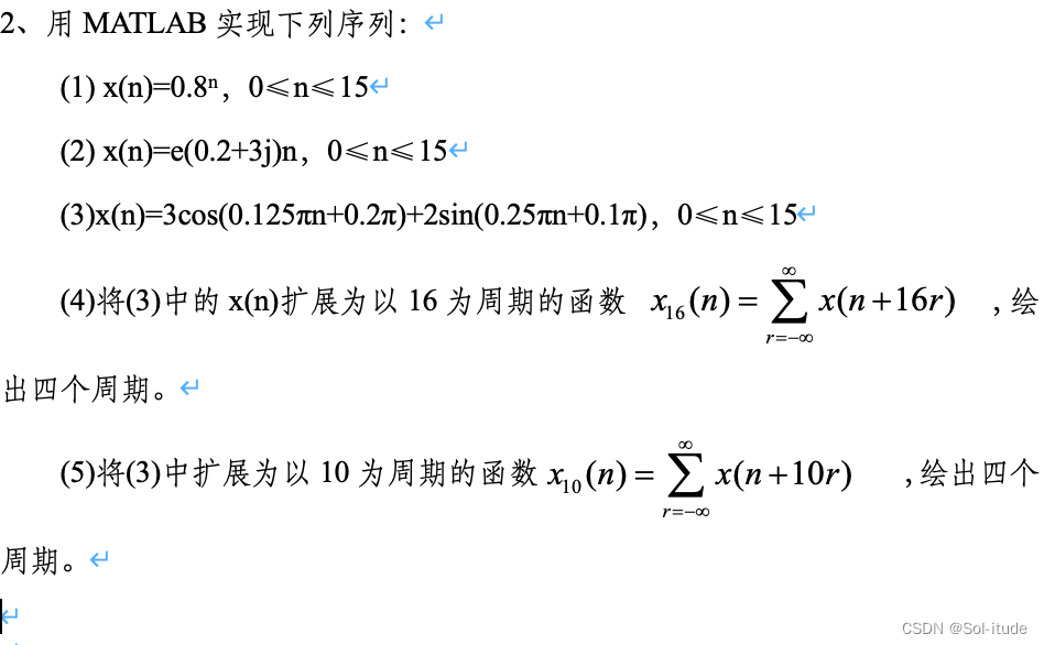
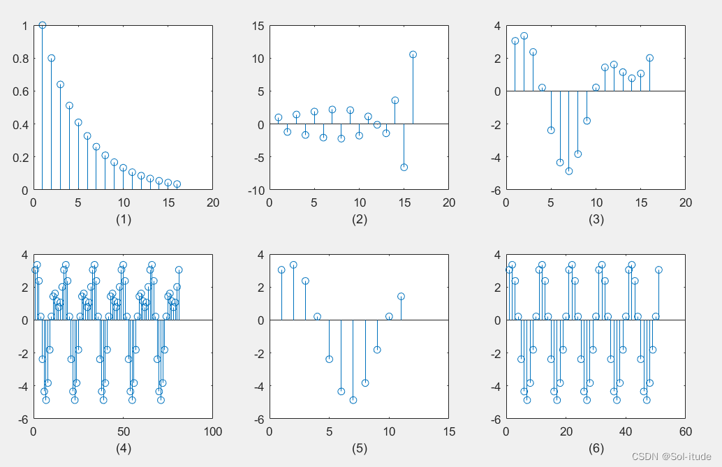
为了看得更清楚我多画了一个(5),是(3)的以10为周期
1
2
3
4
5
6
7
8
9
10
11
12
13
14
15
16
17
18
19
20
21
22
23
24
25
26
27
28
29
30
31
32
33
34
35
36
37
38
39
40
41
| clear;
close all;
clc;
n1=0:15;
x1=0.8.^n1
subplot(2,3,1)
stem(x1)
xlabel('(1)')
n2=0:15;
x2=exp((0.2+3*i)*n2);
subplot(2,3,2)
stem(x2)
xlabel('(2)')
n3=0:15;
x3=3*cos(0.125*pi*n3+0.2*pi)+2*sin(0.25*pi*n3+0.1*pi);
subplot(2,3,3)
stem(x3)
xlabel('(3)')
n4=0:80
n44=mod(n4,16);
x4=3*cos(0.125*pi*n44+0.2*pi)+2*sin(0.25*pi*n44+0.1*pi);
subplot(2,3,4)
stem(x4)
xlabel('(4)')
n5=0:10
x5=3*cos(0.125*pi*n5+0.2*pi)+2*sin(0.25*pi*n5+0.1*pi);
subplot(2,3,5)
stem(x5)
xlabel('(5)')
n6=0:50
n66=mod(n6,10)
x6=3*cos(0.125*pi*n66+0.2*pi)+2*sin(0.25*pi*n66+0.1*pi);
subplot(2,3,6)
stem(x6)
xlabel('(6)')
|
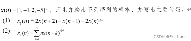
(1)
1
2
3
4
5
6
7
8
9
| clear;
close all;
clc;
n=0:3;
x=[1 -1 2 -5];
x1=2*circshift(x,[0 -2])-circshift(x,[0 1])-2*x;
stem(x1)
xlabel('时间序列n')
|
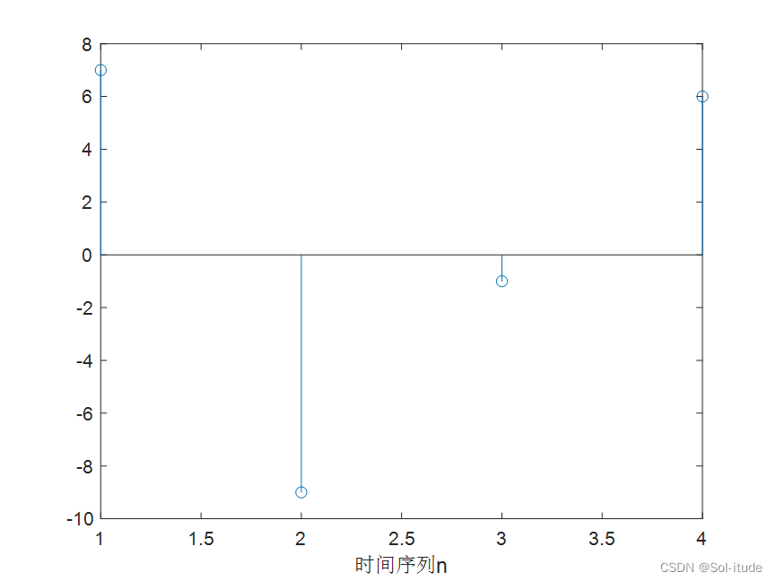
(2)
1
2
3
4
5
6
7
8
9
10
11
12
13
14
| clear;
close all;
clc;
n=0:3;
x=[1 -1 2 -5];
x1=circshift(x,[0 1]);
x2=circshift(x,[0 2]);
x3=circshift(x,[0 3]);
x4=circshift(x,[0 4]);
x5=circshift(x,[0 5]);
xn=1*x1+2*x2+3*x3+4*x4+5*x5;
stem(xn)
xlabel('时间序列n')
|
1
2
3
4
5
6
7
8
9
10
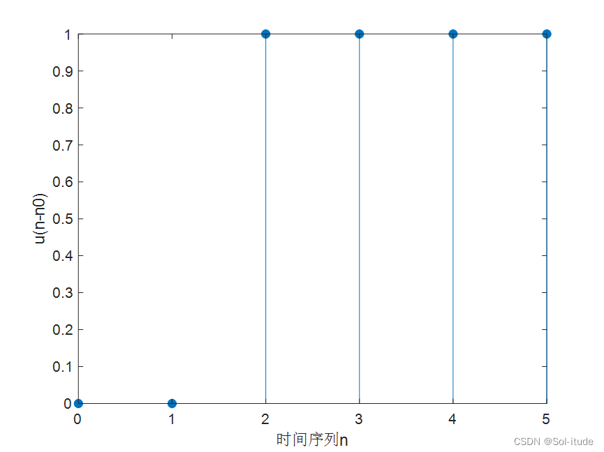
| function stepshift
clc;
n1=input('请输入起点: ');
n2=input('请输入终点:');
n0=input('请输入阶跃位置:');
n=n1:n2;
x=[n-n0>=0];
stem(n,x,'fill');xlabel('时间序列n');ylabel('u(n-n0)');
end
|
1
2
3
4
5
6
7
8
9
10
11
12
13
14
15
16
17
18
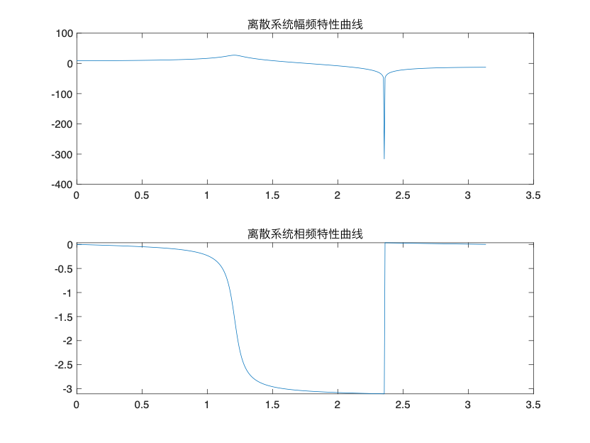
| clear;
close all;
clc;
B=[1 sqrt(2) 1];
A=[1 -0.67 0.9];
[H,w]=freqz(B,A);
Hf=abs(H); %取幅度值实部
Hx=angle(H); %取相位值对应相位角
clf;
subplot(2,1,1)
plot(w,20*log10(Hf)) %幅值变换为分贝单位
title('离散系统幅频特性曲线')
subplot(2,1,2)
plot(w,Hx)
title('离散系统相频特性曲线')
|

1
2
3
4
5
6
7
8
9
10
11
12
13
14
15
16
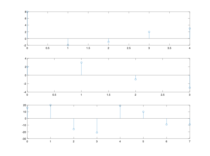
| clear;
close all;
clc;
na=0:4;
nb=0:3;
n=0:7;
A=[8 -2 -1 2 3];
B=[2 3 -1 -3];
subplot(3,1,1)
stem(na,A)
subplot(3,1,2)
stem(nb,B)
C=conv(A,B);
subplot(3,1,3)
stem(n,C)
|